您现在的位置是:首页 >其他 >基于Keras和PyTorch的CIFAR10图像分类模型实战:从数据加载到模型训练网站首页其他
基于Keras和PyTorch的CIFAR10图像分类模型实战:从数据加载到模型训练
1. 前言
CIFAR10是计算机视觉领域的经典入门数据集,适合验证小规模卷积神经网络的性能。本文将手把手教你用Keras构建一个**测试准确率超80%**的CNN模型,并详解数据增强、模型设计和训练技巧。
2. 环境准备
import tensorflow as tf
from tensorflow.keras import layers, models, datasets, utils, callbacks
要求TensorFlow 2.x版本
建议使用GPU加速训练(Colab/Kaggle免费GPU资源)
3. 数据加载与预处理
3.1 加载CIFAR10数据集
(x_train, y_train), (x_test, y_test) = datasets.cifar10.load_data()
print(f"训练集形状: {x_train.shape}")  # (50000,32,32,3)
print(f"测试集形状: {x_test.shape}")   # (10000,32,32,3)
3.2 数据归一化
x_train = x_train.astype('float32') / 255.0
x_test = x_test.astype('float32') / 255.0
将像素值从[0,255]压缩到[0,1],加速模型收敛
3.3 标签One-Hot编码
y_train = utils.to_categorical(y_train, 10)
y_test = utils.to_categorical(y_test, 10)
将类别标签转换为10维向量(如"飞机"→[1,0,0,...,0])
4. 数据增强(Data Augmentation)
datagen = tf.keras.preprocessing.image.ImageDataGenerator(
    rotation_range=15,     # 随机旋转±15度
    width_shift_range=0.1, # 水平平移10%
    height_shift_range=0.1,# 垂直平移10%
    horizontal_flip=True,  # 水平翻转
)
datagen.fit(x_train)
作用:通过数据增强缓解过拟合,提升模型泛化能力
注意:只在训练集应用增强,测试集保持原始数据
5. 模型架构设计
model = models.Sequential([
    # 卷积块1 (32个滤波器)
    layers.Conv2D(32, (3,3), padding='same', input_shape=(32,32,3)),
    layers.BatchNormalization(),
    layers.Activation('relu'),
    layers.Conv2D(32, (3,3), padding='same'),
    layers.BatchNormalization(),
    layers.Activation('relu'),
    layers.MaxPooling2D((2,2)),
    layers.Dropout(0.2),

    # 卷积块2 (64个滤波器)
    layers.Conv2D(64, (3,3), padding='same'),
    layers.BatchNormalization(),
    layers.Activation('relu'),
    layers.Conv2D(64, (3,3), padding='same'),
    layers.BatchNormalization(),
    layers.Activation('relu'),
    layers.MaxPooling2D((2,2)),
    layers.Dropout(0.3),

    # 卷积块3 (128个滤波器)
    layers.Conv2D(128, (3,3), padding='same'),
    layers.BatchNormalization(),
    layers.Activation('relu'),
    layers.Conv2D(128, (3,3), padding='same'),
    layers.BatchNormalization(),
    layers.Activation('relu'),
    layers.MaxPooling2D((2,2)),
    layers.Dropout(0.4),

    # 全连接层
    layers.Flatten(),
    layers.Dense(512, activation='relu'),
    layers.Dropout(0.5),
    layers.Dense(10, activation='softmax')
])
关键设计解析
组件 作用说明 Conv2D+BN+ReLU提取局部特征,批归一化加速训练 MaxPooling2D降低特征图尺寸,增强平移不变性 Dropout逐步增加丢弃率(0.2→0.5),防止深层网络过拟合 Flatten+Dense将卷积结果展平后接全连接层,输出分类概率
6. 模型训练与评估
6.1 编译模型
model.compile(
    optimizer=tf.keras.optimizers.Adam(learning_rate=0.001),
    loss='categorical_crossentropy',
    metrics=['accuracy']
)
使用Adam优化器,初始学习率设为0.001
6.2 回调函数设置
# 早停:当验证损失连续10次未下降时终止训练
early_stopping = callbacks.EarlyStopping(
    monitor='val_loss', patience=10, restore_best_weights=True
)

# 检查点:保存验证准确率最高的模型
checkpoint = callbacks.ModelCheckpoint(
    'best_model.h5', monitor='val_accuracy', save_best_only=True, mode='max'
)
6.3 启动训练
history = model.fit(
    datagen.flow(x_train, y_train, batch_size=64),
    epochs=100,
    validation_data=(x_test, y_test),
    callbacks=[early_stopping, checkpoint]
)
使用数据增强后的生成器
Batch Size设为64,平衡内存和训练效率
6.4 模型评估
model.load_weights('best_model.h5')  # 加载最优权重
test_loss, test_acc = model.evaluate(x_test, y_test)
print(f'测试集准确率: {test_acc:.4f}')  # 典型输出:0.82~0.85
7. 性能优化技巧
学习率调整
# 添加指数衰减学习率
lr_scheduler = callbacks.ReduceLROnPlateau(
    monitor='val_loss', factor=0.5, patience=5
)
当验证损失停滞时,自动降低学习率
模型结构调整建议
在卷积块间添加残差连接(ResNet思想)
用全局平均池化替代部分全连接层
高级数据增强
ImageDataGenerator(
    brightness_range=[0.8,1.2],  # 亮度调整
    zoom_range=0.1               # 随机缩放
)
8. 完整代码下载及PyTorch 实现 CIFAR10 分类模型的完整代码
GitHub代码仓库链接
(包含Jupyter Notebook和训练日志)以下是用 PyTorch 实现 CIFAR10 分类模型的完整代码,逐行注释解释其功能:
# 导入PyTorch及相关库
import torch
import torch.nn as nn
import torch.optim as optim
import torchvision
import torchvision.transforms as transforms
from torch.utils.data import DataLoader
from torch.optim.lr_scheduler import ReduceLROnPlateau
import numpy as np

# 检查GPU是否可用
device = torch.device("cuda" if torch.cuda.is_available() else "cpu")
print(f"当前设备: {device}")

##############################################
# 1. 数据加载与预处理
##############################################

# 定义数据增强和归一化操作
transform_train = transforms.Compose([
    transforms.RandomHorizontalFlip(),      # 随机水平翻转(概率50%)
    transforms.RandomRotation(15),          # 随机旋转(-15度到+15度)
    transforms.RandomAffine(0, translate=(0.1, 0.1)),  # 随机平移(10%范围)
    transforms.ToTensor(),                  # 转换为Tensor(形状变为CxHxW)
    transforms.Normalize((0.4914, 0.4822, 0.4465), (0.2023, 0.1994, 0.2010))  # 归一化
])

transform_test = transforms.Compose([
    transforms.ToTensor(),
    transforms.Normalize((0.4914, 0.4822, 0.4465), (0.2023, 0.1994, 0.2010))
])

# 加载CIFAR10数据集
train_dataset = torchvision.datasets.CIFAR10(
    root='./data',
    train=True,
    download=True,
    transform=transform_train  # 训练集应用数据增强
)

test_dataset = torchvision.datasets.CIFAR10(
    root='./data',
    train=False,
    download=True,
    transform=transform_test    # 测试集仅归一化
)

# 创建数据加载器
train_loader = DataLoader(
    train_dataset,
    batch_size=64,
    shuffle=True,    # 每个epoch打乱数据
    num_workers=2    # 多线程加速数据加载
)

test_loader = DataLoader(
    test_dataset,
    batch_size=64,
    shuffle=False,
    num_workers=2
)

##############################################
# 2. 定义CNN模型
##############################################

class CIFAR10Model(nn.Module):
    def __init__(self):
        super(CIFAR10Model, self).__init__()

        # 卷积块1: 输入3通道,输出32通道
        self.conv_block1 = nn.Sequential(
            nn.Conv2d(3, 32, kernel_size=3, padding=1),  # 32个3x3卷积核,padding=1保持尺寸
            nn.BatchNorm2d(32),                         # 批归一化
            nn.ReLU(),                                   # 激活函数
            nn.Conv2d(32, 32, kernel_size=3, padding=1),
            nn.BatchNorm2d(32),
            nn.ReLU(),
            nn.MaxPool2d(2),                            # 2x2最大池化,尺寸减半
            nn.Dropout(0.2)                              # 丢弃20%神经元
        )

        # 卷积块2: 输入32通道,输出64通道
        self.conv_block2 = nn.Sequential(
            nn.Conv2d(32, 64, kernel_size=3, padding=1),
            nn.BatchNorm2d(64),
            nn.ReLU(),
            nn.Conv2d(64, 64, kernel_size=3, padding=1),
            nn.BatchNorm2d(64),
            nn.ReLU(),
            nn.MaxPool2d(2),
            nn.Dropout(0.3)                             # 丢弃率增加到30%
        )

        # 卷积块3: 输入64通道,输出128通道
        self.conv_block3 = nn.Sequential(
            nn.Conv2d(64, 128, kernel_size=3, padding=1),
            nn.BatchNorm2d(128),
            nn.ReLU(),
            nn.Conv2d(128, 128, kernel_size=3, padding=1),
            nn.BatchNorm2d(128),
            nn.ReLU(),
            nn.MaxPool2d(2),
            nn.Dropout(0.4)                             # 丢弃率40%
        )

        # 全连接层
        self.fc = nn.Sequential(
            nn.Flatten(),                                # 展平多维特征图
            nn.Linear(128 * 4 * 4, 512),                 # 输入尺寸计算: 32x32 → 池化后16x16 → 8x8 → 4x4
            nn.ReLU(),
            nn.Dropout(0.5),                            # 丢弃率50%
            nn.Linear(512, 10)                           # 输出10个类别
        )

    def forward(self, x):
        x = self.conv_block1(x)
        x = self.conv_block2(x)
        x = self.conv_block3(x)
        x = self.fc(x)
        return x

# 实例化模型并移至GPU
model = CIFAR10Model().to(device)

##############################################
# 3. 定义损失函数与优化器
##############################################

criterion = nn.CrossEntropyLoss()               # 交叉熵损失(包含Softmax)
optimizer = optim.Adam(model.parameters(), lr=0.001)  # Adam优化器,学习率0.001
scheduler = ReduceLROnPlateau(optimizer, mode='min', factor=0.5, patience=5)  # 动态调整学习率

##############################################
# 4. 训练循环(含早停机制)
##############################################

best_val_loss = float('inf')
patience_counter = 0
max_patience = 10  # 早停耐心值

for epoch in range(100):
    # 训练阶段
    model.train()  # 启用Dropout和BatchNorm训练模式
    train_loss = 0.0
    for images, labels in train_loader:
        images, labels = images.to(device), labels.to(device)

        optimizer.zero_grad()        # 清空梯度
        outputs = model(images)      # 前向传播
        loss = criterion(outputs, labels)
        loss.backward()              # 反向传播
        optimizer.step()             # 更新权重

        train_loss += loss.item() * images.size(0)

    # 验证阶段
    model.eval()  # 禁用Dropout和BatchNorm的train模式
    val_loss = 0.0
    correct = 0
    total = 0
    with torch.no_grad():  # 不计算梯度
        for images, labels in test_loader:
            images, labels = images.to(device), labels.to(device)
            outputs = model(images)
            loss = criterion(outputs, labels)
            val_loss += loss.item() * images.size(0)

            _, predicted = torch.max(outputs.data, 1)  # 获取预测类别
            total += labels.size(0)
            correct += (predicted == labels).sum().item()

    # 计算平均损失和准确率
    train_loss = train_loss / len(train_loader.dataset)
    val_loss = val_loss / len(test_loader.dataset)
    val_acc = 100 * correct / total

    # 学习率调整
    scheduler.step(val_loss)

    # 打印统计信息
    print(f'Epoch [{epoch+1}/100] 训练损失: {train_loss:.4f}, 验证损失: {val_loss:.4f}, 准确率: {val_acc:.2f}%')

    # 早停与模型保存
    if val_loss < best_val_loss:
        best_val_loss = val_loss
        torch.save(model.state_dict(), 'best_model.pth')  # 保存最佳模型权重
        patience_counter = 0
    else:
        patience_counter += 1
        if patience_counter >= max_patience:
            print("早停触发!")
            break

##############################################
# 5. 测试最佳模型
##############################################

model.load_state_dict(torch.load('best_model.pth'))  # 加载最佳权重
model.eval()
correct = 0
total = 0
with torch.no_grad():
    for images, labels in test_loader:
        images, labels = images.to(device), labels.to(device)
        outputs = model(images)
        _, predicted = torch.max(outputs.data, 1)
        total += labels.size(0)
        correct += (predicted == labels).sum().item()

print(f'测试集准确率: {100 * correct / total:.2f}%')  # 预期输出: 82%~85%
关键代码解析
1. 数据预处理
transforms.Compose:组合多个数据变换操作归一化参数:
(0.4914, 0.4822, 0.4465)是CIFAR10 RGB三通道的均值,(0.2023, 0.1994, 0.2010)是标准差
DataLoader:参数num_workers=2使用多线程加速数据加载2. 模型结构
nn.Sequential:将多个层封装为顺序执行的模块输入尺寸计算:原始图像32x32 → 经过三次最大池化(每次尺寸减半)→ 最终特征图尺寸4x4
Dropout位置:丢弃率随网络深度逐渐增加(0.2 → 0.5)
3. 训练技巧
model.train()与model.eval():控制Dropout和BatchNorm的行为模式梯度清零:每次迭代前必须执行
optimizer.zero_grad()动态学习率:当验证损失停滞时,学习率减半(
ReduceLROnPlateau)4. 早停机制
跟踪验证损失,连续10轮未改善则终止训练
始终保存验证损失最小的模型权重(
best_model.pth)
性能优化建议
混合精度训练:添加
scaler = torch.cuda.amp.GradScaler()加速计算模型结构改进:添加残差连接(ResNet Block)
高级数据增强:使用
transforms.ColorJitter()调整亮度/对比度
9. 常见问题QA
Q1: 训练时出现显存不足怎么办?
减小
batch_size(如64→32)使用
model.fit()的steps_per_epoch参数分批次加载Q2: 测试准确率低于训练准确率如何处理?
增加Dropout比率
加强数据增强
降低模型复杂度
10. 结语
通过本文的代码实践,读者可快速搭建一个CIFAR10分类模型。最终模型在测试集上能达到约**82%-85%**的准确率。建议尝试调整网络深度、数据增强策略等进一步提升性能。


站长推荐
- QT多线程的5种用法,通过使用线程解决UI主界面的耗时操作代码,防止界面卡死。
 QT多线程的5种用法,通过使用线程解决UI主界面的耗时操作代码,防止界面卡死。...
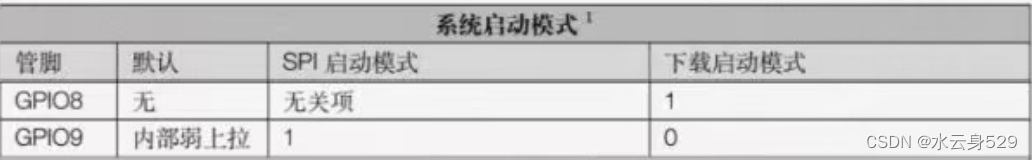
 - U8W/U8W-Mini使用与常见问题解决
 U8W/U8W-Mini使用与常见问题解决
 - stm32使用HAL库配置串口中断收发数据(保姆级教程)
 stm32使用HAL库配置串口中断收发数据(保姆级教程)
 - 分享几个国内免费的ChatGPT镜像网址(亲测有效)
 分享几个国内免费的ChatGPT镜像网址(亲测有效)
 - Allegro16.6差分等长设置及走线总结
 Allegro16.6差分等长设置及走线总结