您现在的位置是：首页 >技术杂谈 >基于python使用Robust最小二乘法和RANSAC方法作直线拟合网站首页技术杂谈

一、原理

1.Robust最小二乘法（Robust Least Squares Method）

        当数据中存在异常值时，最小二乘法的结果可能会受到较大的影响，导致模型的预测精度下降。为了增强对异常值的鲁棒性，Robust最小二乘法采用了不同的损失函数。传统的最小二乘法使用残差平方和作为损失函数，而Robust最小二乘法则使用对异常值不那么敏感的损失函数，如Huber损失、Tukey损失等。这些损失函数在残差较小时与残差平方和相似，但在残差较大时增长较慢，从而减小了异常值对参数估计的影响。

2.RANSAC方法（Random Sample Consensus，随机采样一致性）

        RANSAC方法是一种基于随机采样的迭代算法，主要用于从包含大量噪声和异常值（外点）的数据集中估计数学模型参数。其从数据集中随机选择一组样本点（对于直线拟合，通常需要两个点来确定一条直线），再使用选择的样本点来估计直线模型的参数（斜率和截距），并计算数据集中剩余点到估计直线的距离，将距离小于某个阈值的点视为内点。统计内点的数量，并评估当前模型的质量（通常以内点数量作为评估标准）。重复步骤多次（通常预设一个最大迭代次数），每次迭代都会生成一个新的模型，并选择内点数量最多的模型作为当前最佳模型。当达到最大迭代次数或当前最佳模型的质量不再显著提高时，算法终止，并输出最终的最佳模型。

二、代码

1.Robust最小二乘法

import cv2
import numpy as np
import matplotlib.pyplot as plt
plt.rcParams['font.sans-serif'] = ['SimHei']
plt.rcParams['axes.unicode_minus'] = False

# robust最小二乘法函数
def robust_least_squares(x, y, degree, iterations, epsilon):
    # 初始化参数
    theta = np.zeros(degree + 1)
    m = len(x)
    # 添加偏置项（x^0 = 1）
    X = np.column_stack([np.power(x, i) for i in range(degree + 1)])
    # 迭代更新参数
    for _ in range(iterations):
        # 计算预测值
        y_pred = np.dot(X, theta)
        # 计算残差
        residuals = y - y_pred
        # 计算权重矩阵
        weights = np.diag(1 / (np.abs(residuals) + epsilon))  
        # 更新参数（使用加权最小二乘法）
        theta = np.linalg.inv(X.T @ weights @ X) @ X.T @ weights @ y
    
    return theta

# 读取图像并处理
image = cv2.imread('dot.png')
gray = cv2.cvtColor(image, cv2.COLOR_BGR2GRAY)
_, binary = cv2.threshold(gray, 127, 255, cv2.THRESH_BINARY_INV)
contours, _ = cv2.findContours(binary, cv2.RETR_EXTERNAL, cv2.CHAIN_APPROX_SIMPLE)

# 存储x和y坐标
x_coords = []
y_coords = []

# 遍历轮廓，找到每个点的中心
for contour in contours:
    M = cv2.moments(contour)
    if M["m00"] != 0:
        cX = int(M["m10"] / M["m00"]) / 1000
        cY = (600 - int(M["m01"] / M["m00"])) / 1000
        x_coords.append(cX)
        y_coords.append(cY)

X_data = np.array(x_coords)
y_data = np.array(y_coords)

# 设置多项式的度数、迭代次数和epsilon值
degree = 1  #多项式次数
iterations = 100  # 迭代次数
epsilon = 1e-6  # 避免除以零的小正数

# 使用函数拟合曲线并打印拟合参数
theta_optimal = robust_least_squares(X_data, y_data, degree, iterations, epsilon)
print("Optimal theta values:", theta_optimal)

# 生成用于绘图的x值范围
x_fit = np.linspace(min(X_data), max(X_data), 100).reshape(-1, 1)

# 使用拟合参数计算y值
y_fit = np.dot(np.column_stack([np.power(x_fit, i) for i in range(degree + 1)]), theta_optimal)

# 绘制样本点和拟合曲线
plt.scatter(X_data, y_data, label='数据点')
plt.plot(x_fit, y_fit, color='red', label='拟合曲线')
plt.xlabel('X')
plt.ylabel('Y')
plt.legend()
plt.title('robust最小二乘法拟合')
plt.show()

2.RANSAC方法

import cv2
from copy import copy
import numpy as np
from numpy.random import default_rng
plt.rcParams['font.sans-serif'] = ['SimHei']
plt.rcParams['axes.unicode_minus'] = False

rng = default_rng()

# 定义RANSAC类，用于实现随机抽样一致性算法
class RANSAC:
    def __init__(self, n=10, k=100, t=0.05, d=10, model=None, loss=None, metric=None):
        # 初始化参数
        self.n = n  # 最小数据点数量，用于估计模型参数
        self.k = k  # 最大迭代次数
        self.t = t  # 阈值，用于确定点是否拟合良好
        self.d = d  # 所需接近数据点的数量，以确认模型拟合良好
        self.model = model  # 模型类，实现fit和predict方法
        self.loss = loss  # 损失函数，返回y_true和y_pred之间的向量
        self.metric = metric  # 度量函数，返回y_true和y_pred之间的浮点数
        self.best_fit = None  # 最佳拟合模型
        self.best_error = np.inf  # 最佳误差，初始化为无穷大

    def fit(self, X, y):
        # 对数据进行RANSAC拟合
        for _ in range(self.k):
            ids = rng.permutation(X.shape[0])# 对数据点进行随机排列

            maybe_inliers = ids[: self.n]# 选择前n个点作为可能的内点
            maybe_model = copy(self.model).fit(X[maybe_inliers], y[maybe_inliers])# 使用这些点拟合模型
            # 计算剩余点的损失，并确定哪些点满足阈值条件
            thresholded = (
                self.loss(y[ids][self.n :], maybe_model.predict(X[ids][self.n :]))
                < self.t
            )

            inlier_ids = ids[self.n :][np.flatnonzero(thresholded).flatten()]# 获取满足条件的内点索引
            # 如果内点数量足够，则更新模型
            if inlier_ids.size > self.d:
                inlier_points = np.hstack([maybe_inliers, inlier_ids])# 合并可能的内点和实际的内点
                better_model = copy(self.model).fit(X[inlier_points], y[inlier_points])# 使用所有内点重新拟合模型

                this_error = self.metric(
                    y[inlier_points], better_model.predict(X[inlier_points])# 计算当前模型的误差
                )
                # 如果当前模型的误差更小，则更新最佳拟合模型和最佳误差
                if this_error < self.best_error:
                    self.best_error = this_error
                    self.best_fit = maybe_model

        return self

    def predict(self, X):
        return self.best_fit.predict(X) # 使用最佳拟合模型进行预测

# 定义损失函数和度量函数
def square_error_loss(y_true, y_pred):
    return (y_true - y_pred) ** 2   # 计算平方误差损失

def mean_square_error(y_true, y_pred):
    return np.sum(square_error_loss(y_true, y_pred)) / y_true.shape[0]  # 计算均方误差

# 定义线性回归模型类
class LinearRegressor:
    def __init__(self):
        self.params = None

    def fit(self, X: np.ndarray, y: np.ndarray):
        # 拟合线性回归模型
        r, _ = X.shape
        X = np.hstack([np.ones((r, 1)), X])
        self.params = np.linalg.inv(X.T @ X) @ X.T @ y
        return self

    def predict(self, X: np.ndarray):
        # 使用线性回归模型进行预测
        r, _ = X.shape
        X = np.hstack([np.ones((r, 1)), X])
        return X @ self.params

if __name__ == "__main__":
    # 创建RANSAC实例，使用线性回归模型和定义的损失函数、度量函数
    regressor = RANSAC(model=LinearRegressor(), loss=square_error_loss, metric=mean_square_error)

    # 读取图像
    image = cv2.imread('dot.png')
    # 转换为灰度图像
    gray = cv2.cvtColor(image, cv2.COLOR_BGR2GRAY)
    # 应用二值化
    _, binary = cv2.threshold(gray, 127, 255, cv2.THRESH_BINARY_INV)
    # 找到轮廓（这里假设点是小而圆的，因此可以使用findContours）
    contours, _ = cv2.findContours(binary, cv2.RETR_EXTERNAL, cv2.CHAIN_APPROX_SIMPLE)

    # 存储x和y坐标
    x_coords = []
    y_coords = []

    # 遍历轮廓，找到每个点的中心
    for contour in contours:
        # 计算轮廓的矩
        M = cv2.moments(contour)
        if M["m00"] != 0:
            # 使用矩来计算中心
            cX = int(M["m10"] / M["m00"])/1000
            cY = (600-int(M["m01"] / M["m00"]))/1000
            x_coords.append(cX)
            y_coords.append(cY)

    # 将坐标转换为NumPy数组
    X = np.array(x_coords).reshape(-1, 1)  # 现在x是一个二维数组，每行一个x坐标
    y = np.array(y_coords).reshape(-1, 1)

    # 拟合模型
    regressor.fit(X, y)

    import matplotlib.pyplot as plt
    fig, ax = plt.subplots(1, 1)
    ax.set_box_aspect(1)
    
    plt.scatter(X, y, label='数据点')
    line = np.linspace(-1, 1, num=100).reshape(-1, 1)
    plt.plot(line, regressor.predict(line), c="peru", label='拟合曲线')
    # 设置坐标轴范围
    plt.xlim(0, 1)
    plt.ylim(0, 1)
    plt.legend()
    plt.title('RANSAC方法拟合直线')
    plt.show()

三、效果

1.Robust最小二乘法

原图：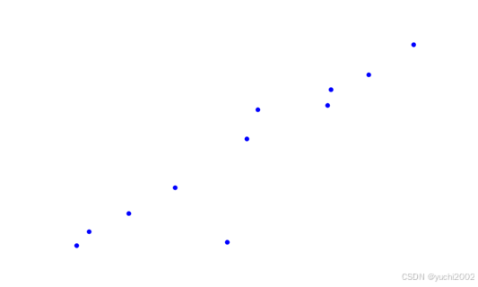

结果：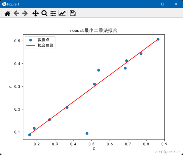

2.RANSAC方法

原图：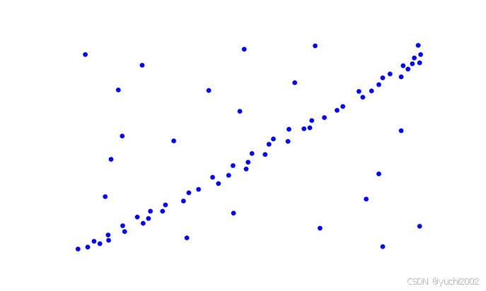

结果：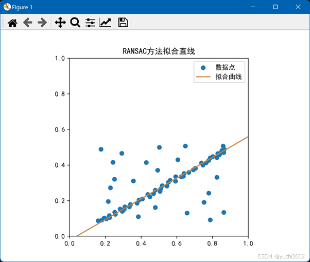

PS:画点函数

随手没有技术含量的画点函数

import numpy as np
import matplotlib.pyplot as plt

# 给定的坐标数据
X = np.array([-0.9,-0.83,-0.61,-0.35,-0.06,0.52,0.73,0.98,0.11,0.50,0.05]).reshape(-1, 1)
y = np.array([-0.93,-0.80,-0.63,-0.39,-0.9,0.53,0.67,0.95,0.34,0.38,0.07]).reshape(-1, 1)

# 创建图形和轴
plt.figure(figsize=(10, 6))

# 绘制散点图
plt.scatter(X, y, color='blue')#, label='Data Points'

# 添加标题和标签
# plt.title('Scatter Plot of X and y')
# plt.xlabel('X')
# plt.ylabel('y')
# plt.legend()
plt.axis('off')

# 保存图像到文件
plt.savefig('dot.png')

# 显示图形（可选，如果你想要立即看到图形）
# plt.show()