您现在的位置是:首页 >技术教程 >tensorflow深度神经网络实现鸢尾花分类网站首页技术教程
tensorflow深度神经网络实现鸢尾花分类
tensorflow深度神经网络实现鸢尾花分类
本文目录
获取数据集
下载鸢尾花数据集:https://gitcode.net/mirrors/mwaskom/seaborn-data

相关库的导入
import tensorflow as tf
# 绘图
import seaborn as sns
# 数值计算
import numpy as np
# sklearn中的相关工具
# 划分训练集和测试集
from sklearn.model_selection import train_test_split
import matplotlib.pyplot as plt
from sklearn.metrics import accuracy_score, classification_report
数据展示和划分
利用seaborn导入相关的数据,iris数据以dataFrame的方式在seaborn进行存储,我们读取后并进行展示
# 读取数据
# iris = sns.load_dataset("iris")
iris = sns.load_dataset("iris", cache=True, data_home='./seaborn-data/')
# 展示数据的前五行
print(iris.head())
   sepal_length  sepal_width  petal_length  petal_width species
0           5.1          3.5           1.4          0.2  setosa
1           4.9          3.0           1.4          0.2  setosa
2           4.7          3.2           1.3          0.2  setosa
3           4.6          3.1           1.5          0.2  setosa
4           5.0          3.6           1.4          0.2  setosa
利用seaborn中pairplot函数探索数据特征间的关系
# 将数据之间的关系进行可视化
sns.pairplot(iris, hue='species')
plt.show()
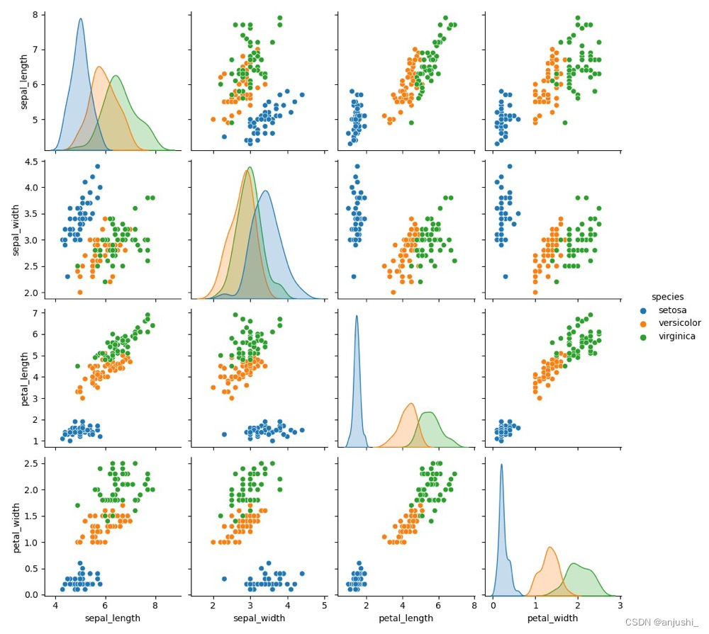
从iris dataframe中提取原始数据,将花瓣和萼片数据保存在数组X中,标签保存在相应的数组y中
# 花瓣和花萼的数据
X = iris.values[:, :4]
# 标签值
y = iris.values[:, 4]
利用train_test_split将数据划分为训练集和测试集
# 将数据集划分为训练集和测试集
train_X, test_X, train_y, test_y = train_test_split(X, y, train_size=0.7, test_size=0.3, random_state=0)s
对标签值进行热编码
独热编码:将分类变量转换为一组二进制变量的过程,其中每个二进制变量对应一个分类变量的值。这些二进制变量中的一个包含“1”,其余变量都包含“0”。这些二进制变量可以被视为一组互斥的指示器,因此独热编码也称为“一位有效编码”(One-of-N Encoding)

# 进行独热编码
def one_hot_encode_object_array(arr):
    # 去重获取全部的类别
    uniques, ids = np.unique(arr, return_inverse=True)
    # 返回热编码的结果
    return tf.keras.utils.to_categorical(ids, len(uniques))


# 训练集热编码
train_y_ohe = one_hot_encode_object_array(train_y)
# 测试集热编码
test_y_ohe = one_hot_encode_object_array(test_y)
模型搭建
tf.Keras是一个神经网络库,我们需要根据数据和标签值构建神经网络。神经网络可以发现特征与标签之间的复杂关系。神经网络是一个高度结构化的图,其中包含一个或多个隐藏层。每个隐藏层都包含一个或多个神经元。神经网络有多种类别,该程序使用的是密集型神经网络,也称为全连接神经网络:一个层中的神经元将从上一层中的每个神经元获取输入连接。
一个密集型神经网络,其中包含 1 个输入层、2 个隐藏层以及 1 个输出层,如下图所示:
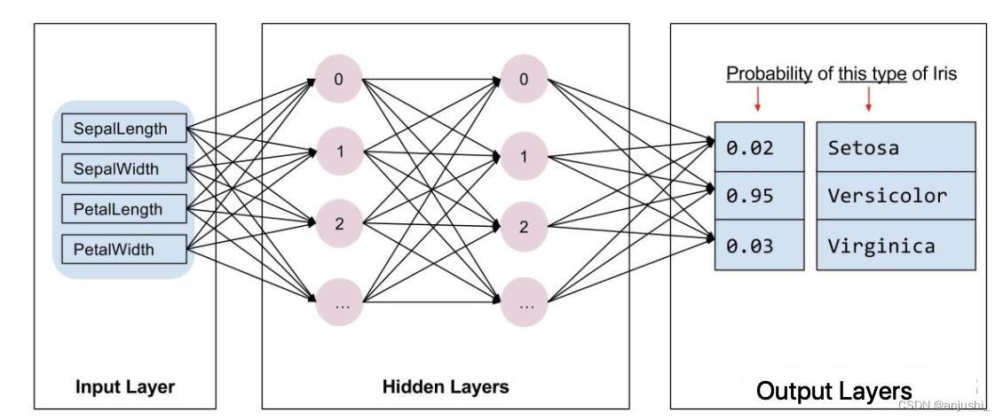
上图 中的模型经过训练并馈送未标记的样本时,它会产生 3 个预测结果:相应鸢尾花属于指定品种的可能性。对于该示例,输出预测结果的总和是 1.0。该预测结果分解如下:山鸢尾为 0.02,变色鸢尾为 0.95,维吉尼亚鸢尾为 0.03。这意味着该模型预测某个无标签鸢尾花样本是变色鸢尾的概率为 95%
使用Sequential模型
搭建模型
tf.keras.Sequential 模型是层的线性堆叠,采用的是 2 个密集层(分别包含 10 个节点)以及 1 个输出层(包含 3 个代表标签预测的节点)。第一个层的 input_shape 参数对应该数据集中的特征数量
# 利用sequential方式构建模型
model = tf.keras.models.Sequential([
    # 隐藏层1,激活函数是relu,输入大小有input_shape指定
    tf.keras.layers.Dense(10, activation="relu", input_shape=(4,)),
    # 隐藏层2,激活函数是relu
    tf.keras.layers.Dense(10, activation="relu"),
    # 输出层
    tf.keras.layers.Dense(3, activation="softmax")
])
查看模型的架构
model.summary()
Model: "sequential"
_________________________________________________________________
 Layer (type)                Output Shape              Param #
=================================================================
 dense (Dense)               (None, 10)                50

 dense_1 (Dense)             (None, 10)                110

 dense_2 (Dense)             (None, 3)                 33

=================================================================
Total params: 193
Trainable params: 193
Non-trainable params: 0
_________________________________________________________________
模型训练
设置优化策略和损失函数,以及模型精度的计算方法
# 设置模型的相关参数:优化器,损失函数和评价指标
model.compile(optimizer='adam',
              loss='categorical_crossentropy',
              metrics=['accuracy'],
)
- 迭代每个epoch。通过一次数据集即为一个epoch。
- 在一个epoch中,遍历训练 Dataset 中的每个样本,并获取样本的特征 (x) 和标签 (y)。
- 根据样本的特征进行预测,并比较预测结果和标签。衡量预测结果的不准确性,并使用所得的值计算模型的损失和梯度。
- 使用 optimizer 更新模型的变量。
- 对每个epoch重复执行以上步骤,直到模型训练完成。
# 模型训练:epochs,训练样本送入到网络中的次数,batch_size:每次训练的送入到网络中的样本个数
history = model.fit(train_X, train_y_ohe, epochs=100, batch_size=1, verbose=1, validation_data=(test_X, test_y_ohe))
训练过程
...
105/105 [==============================] - 1s 7ms/sample - loss: 0.0561 - acc: 0.9619 - val_loss: 0.1246 - val_acc: 0.9778
Epoch 97/100
105/105 [==============================] - 1s 6ms/sample - loss: 0.0732 - acc: 0.9524 - val_loss: 0.0941 - val_acc: 0.9778
Epoch 98/100
105/105 [==============================] - 1s 6ms/sample - loss: 0.0566 - acc: 0.9714 - val_loss: 0.1209 - val_acc: 0.9778
Epoch 99/100
105/105 [==============================] - 1s 6ms/sample - loss: 0.0575 - acc: 0.9810 - val_loss: 0.1297 - val_acc: 0.9556
Epoch 100/100
105/105 [==============================] - 1s 6ms/sample - loss: 0.0609 - acc: 0.9714 - val_loss: 0.0802 - val_acc: 0.9778
对训练好的模型进行评估
计算损失和准确率
# 输出模型评估报告
y_pred = model.predict(test_X)
print('Accuracy score:', accuracy_score(test_y_ohe.argmax(axis=1), y_pred.argmax(axis=1)))
print(classification_report(test_y_ohe.argmax(axis=1), y_pred.argmax(axis=1)))
Accuracy score: 0.9777777777777777
              precision    recall  f1-score   support

           0       1.00      1.00      1.00        16
           1       1.00      0.94      0.97        18
           2       0.92      1.00      0.96        11

    accuracy                           0.98        45
   macro avg       0.97      0.98      0.98        45
weighted avg       0.98      0.98      0.98        45
# 获取模型训练过程的准确率以及损失率的变化
accuracy = history.history['acc']
loss = history.history['loss']
val_loss = history.history['val_loss']
val_accuracy = history.history['val_acc']
epochs = range(len(accuracy))
plt.plot(epochs, accuracy, 'b', label='Training accuracy')
plt.plot(epochs, val_accuracy, 'orange', label='Validation accuracy')
plt.title('Training and validation accuracy')
plt.legend()
plt.show()

plt.plot(epochs, loss, 'b', label='Training Loss')
plt.plot(epochs, val_loss, 'orange', label='Validation Loss')
plt.title('Training and validation loss')
plt.legend()
plt.show()


使用model模型
搭建模型
tf.keras 提供了 Functional API,建立更为复杂的模型,使用方法是将层作为可调用的对象并返回张量,并将输入向量和输出向量提供给 tf.keras.Model 的 inputs 和 outputs 参数
inputs = tf.keras.Input(shape=(4,))
x = tf.keras.layers.Dense(10, activation="relu")(inputs)
x = tf.keras.layers.Dense(10, activation="relu")(x)
outputs = tf.keras.layers.Dense(3, activation="softmax")(x)
model = tf.keras.Model(inputs=inputs, outputs=outputs)
可以优化,正则化通过对算法的修改来减少泛化误差
x = tf.keras.layers.Dense(10, activation="relu", kernel_regularizer=tf.keras.regularizers.l2(0.01))(inputs)
x = tf.keras.layers.Dense(10, activation="relu", kernel_regularizer=tf.keras.regularizers.l2(0.01))(x)
Model: "model"
_________________________________________________________________
 Layer (type)                Output Shape              Param #
=================================================================
 input_1 (InputLayer)        [(None, 4)]               0

 dense (Dense)               (None, 10)                50

 dense_1 (Dense)             (None, 10)                110

 dense_2 (Dense)             (None, 3)                 33

=================================================================
Total params: 193
Trainable params: 193
Non-trainable params: 0
_________________________________________________________________
对训练好的模型进行评估
Accuracy score: 0.9777777777777777
              precision    recall  f1-score   support

           0       1.00      1.00      1.00        14
           1       1.00      0.94      0.97        17
           2       0.93      1.00      0.97        14

    accuracy                           0.98        45
   macro avg       0.98      0.98      0.98        45
weighted avg       0.98      0.98      0.98        45
损失函数
-
分类任务
- 多分类任务:softmax
- 二分类:sigmoid
-
回归任务
-
MAE:Mean absolute loss(MAE)也被称为L1 Loss,以绝对误差作为距离
-
MSE:Mean Squared Loss/ Quadratic Loss(MSE loss)也被称为L2 loss,或欧氏距离,以误差的平方和作为距离
-
smooth L1

-
优化方法
-
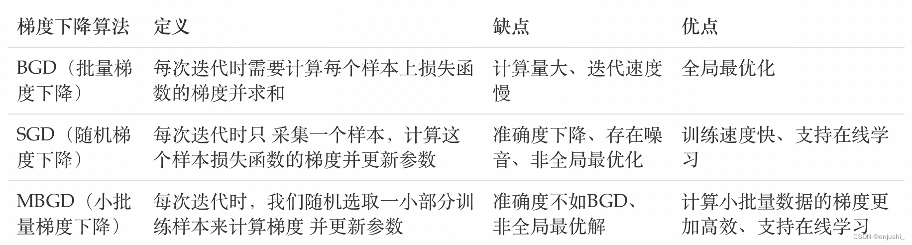
梯度下降
-
反向传播算法(BP算法)
-
梯度下降优化方法
- 动量算法(Momentum)
- AdaGrad
- RMSprop
- Adam
-
学习率退火
正则化
- L1正则化
- L2正则化
- L1L2
- Dropout正则化
- 提前停止


站长推荐
- QT多线程的5种用法,通过使用线程解决UI主界面的耗时操作代码,防止界面卡死。
 QT多线程的5种用法,通过使用线程解决UI主界面的耗时操作代码,防止界面卡死。...
 - U8W/U8W-Mini使用与常见问题解决
 U8W/U8W-Mini使用与常见问题解决
 - stm32使用HAL库配置串口中断收发数据(保姆级教程)
 stm32使用HAL库配置串口中断收发数据(保姆级教程)
 - 分享几个国内免费的ChatGPT镜像网址(亲测有效)
 分享几个国内免费的ChatGPT镜像网址(亲测有效)
 - Allegro16.6差分等长设置及走线总结
 Allegro16.6差分等长设置及走线总结